Measuring how long things take is harder than it seems

Measuring how long a process takes seems easy: start, stop, average. So it should disturb you to find out there’s an entire subfield of statistics devoted to it.

This post looks at why time-to-event data is trickier than it seems and the mistakes people commonly make. If you’d like a more mathematical treatment and a different angle, I also recommend Michał Chorowski’s excellent post on the same topic.

The suspiciously good metric

Imagine you run a team that fixes bugs reported by users. Over a year, you receive bug reports continuously, and each report stays open until the bug is fixed.

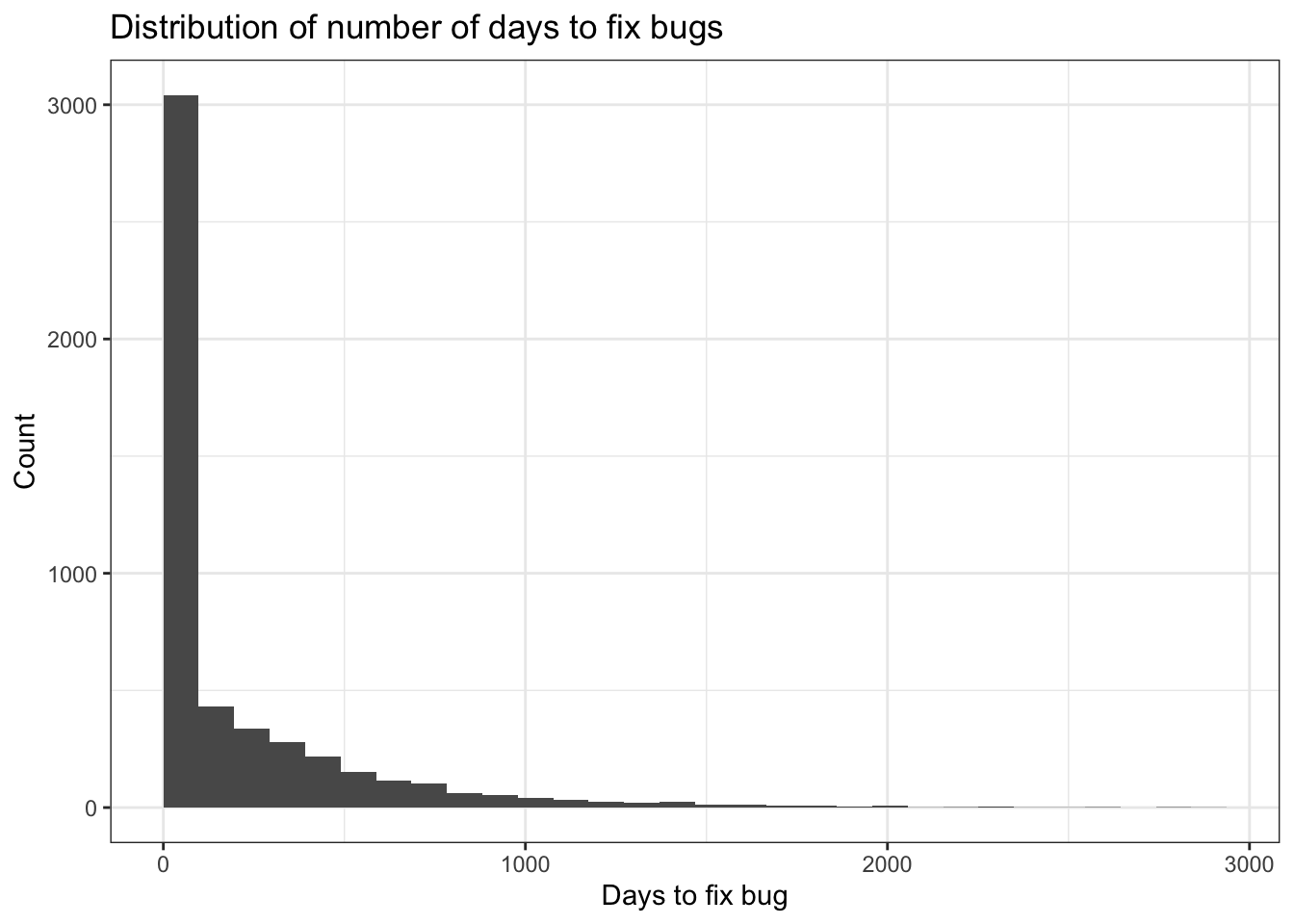
In my simulation, a bug takes a median of 32 days to resolve. But there are really two kinds of bugs: simple ones that are fixed quickly (median 8 days) and complex ones that take much longer (median 272 days). For simplicity, assume you receive equal numbers of simple and complex bugs.

The plot below shows the distribution of time to fix bugs, giving a sense of how much variability there is.

Now it’s the end of the year and you need to report on how quickly bugs are resolved. The obvious approach is to look at the bugs that were fixed during the year and take the median time taken to fix those. When you do that, you get a median resolution time of 12 days.

But I already told you that in this simulated data the median is actually 32 days. So what’s going on? Why is the reported median so misleadingly low?

Right censoring: why ignoring open cases is a mistake

The reason the naive median is wrong is simple: many complex bugs will still be open at the end of the year. You don’t know how long they will ultimately take to resolve, because they haven’t resolved yet.

Those unresolved cases are right-censored. An observation is right censored if the event you’re interested in (the bug being fixed) hasn’t happened yet.

Although we don’t yet know exactly how long it will take until the event happens, we still know something. For example, a bug that has been open for 200 days will take at least 200 days to resolve. When we throw out that information, we create a bias in our reported time to resolution. Because we exclude many of the bugs that take longest to fix (since those are most likely to still be open), our naive median is skewed towards shorter durations and paints a misleadingly rosy picture.

One reason these mistakes persist is that they make performance look better than it really is, so they don’t naturally trigger scrutiny. But for a data scientist, an unexpectedly good headline KPI should trigger suspicion rather than celebration.

When timeliness KPIs don’t mean what they seem

Suppose you also have a KPI: 80% of bugs should be resolved within 120 days. That sounds straightforward, but there are at least two different ways people might interpret this:

• Closed case framing: of all the bugs fixed in a time period, 80% were fixed within 120 days
• Intake cohort framing: of all the bugs reported in a time period, 80% were fixed within 120 days

These sound disarmingly similar, but they are actually very different.

When most people hear a statement like “80% of bugs are resolved within 120 days”, they interpret it as a promise about their own experience: if they submit a bug, there’s an 80% chance it will be resolved within 120 days.

But the first framing does not mean that at all. It means that if a bug happens to be resolved during this reporting period, there’s an 80% chance it was resolved within 120 days. That can be true even if the chance my bug is resolved at all is tiny.

If your goal is to communicate something like service standards to users or stakeholders, the second framing is closer to what they think they’re reading.

The backlog is your reality check

When we only include closed bugs, we ignore the backlog. But the backlog contains the most important information.

In the simulation, if you look only at closed bugs you would conclude that performance was excellent: 91% of bugs were fixed within 120 days.

The backlog tells a very different story. At the end of the year, there are 1767 open bug reports, of which 913 (52%) have been open for more than 120 days.

On the face of it, this is hard to reconcile with our headline KPI result. After all, we know that at least 52% of currently open bugs will take more than 120 days to resolve, as they’ve already been open for at least that long.

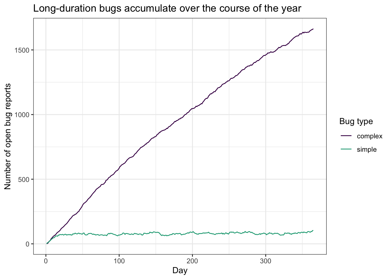
Why does this happen? Because simple bugs are fixed quickly while complex bugs aren’t, and they arrive in similar numbers. Over time, complex bugs accumulate in the backlog. So any metric that conditions on being closed will over-represent quick, simple bugs.

That bias is inevitable. We can see how complex cases accumulate over time in the figure below:

Bad metrics incentivise bad behaviour

As statistically disturbing as this all is, there’s a nastier problem with measuring timeliness based on closed cases only.

Because bugs are effectively invisible until they are closed, closing complex, long duration bugs actually makes your stats worse. Once a bug is already older than 120 days, it can only hurt your “% within 120 days” metric when you close it.

This creates a perverse incentive to never close bugs that are already past the 120-day threshold. A canny but unethical manager could push the KPI to 100% simply by ceasing work on bugs over 120 days old. Any KPI that only counts cases once they’re closed risks rewarding delay on the hardest work. As impressive this will look on a dashboard, user experience will clearly be worse.

Do better

So how do we avoid this? The right metric will always depend on what you’re trying to learn or communicate, but there are a few approaches that reliably avoid the traps above.

1. Use survival modelling

Survival modelling exists specifically to deal with the problem of censored observations. Instead of discarding open bugs, you include them with their current age and an indicator for whether they’ve resolved.

A Kaplan–Meier curve (or a more complex survival model if you need covariates) will incorporate information from open cases rather than throwing it away. Using our simulated data, fitting a Kaplan–Meier curve recovers a median bug resolution time of 32 days. This very closely matches the actual median. Importantly, we arrive at this correct value even though we don’t yet know how long some bugs will ultimately take to fix.

2. Define “% resolved within X days” using an intake cohort

If what you really want to know is “if a bug is reported, what is the probability it’s resolved within 120 days?”, you should define the denominator as all bugs reported in a period rather than all bugs closed in a period.

Using the simulated data, 63% of bug reports that were received were fixed within 120 days. This is much less flattering than the 91% we get using the naive method, but much more representative of reality.

The downside is that you can’t finalise the metric immediately: you need to wait at least 120 days after the reporting period ends to know which bugs made the threshold.

3. If you must use the naive timeliness KPI, always publish backlog metrics alongside it

Sometimes an organisation is locked into a particular KPI definition. This is definitely one worth arguing about why you should do better, but if you’re forced to use timeliness calculated on closed cases only you must at least pair it with backlog reporting.

At minimum, publish the backlog size, whether it’s increasing or decreasing, and the age distribution of open cases (for example: proportion open more than six months, more than one year, more than five years).

Takeaways

If you remember nothing else, remember these three points:

• Any average time to resolve calculated only on resolved cases is biased when there’s a backlog and resolution times are likely to be long.
• A statement like “X% resolved within Y days” is ambiguous unless you specify whether the denominator is cases closed or opened in the period
• If you report a timeliness KPI, also report backlog size and backlog age distribution. If you don’t, you’re hiding the slow cases.

Once you know about right censoring, you’ll see it everywhere: complaint handling, recruitment pipelines, incident response, clinical wait times, and just about any process where the slowest cases are still open when reporting happens. There’s no unseeing it (sorry!).