Automated web scraping using GitLab CI/CD

Author

Gabrielle

Published

July 19, 2021

When working on data projects that rely on regularly updated sources, it’s easy to end up with a manual refresh process — running a series of scripts locally, saving the results, and uploading the new data wherever it’s needed. That approach works fine at first, but quickly becomes repetitive and error-prone as the project grows.

This post describes how I used GitLab CI/CD and AWS S3 to automate a set of R scripts that collect, clean, and process data on a schedule. The outputs are stored in S3 so they can be accessed by any downstream application or analysis without needing to re-run the full pipeline. Because this setup involved a few tools I hadn’t used together before, I’ll go through the key steps I took to get it working reliably.

The original workflow and why it needed to change

The project involved collecting data from an external source that changed frequently. The raw inputs required a fair amount of cleaning and transformation before they were useful. My initial workflow looked something like this:

Run the scraping, cleaning, and processing scripts locally. The resulting R objects were saved to disk.
Push the updated files to a GitLab repository for safekeeping or deployment elsewhere.
Manually copy or pull the updated files into the environment that needed them.

This wasn’t especially complex, but it was time-consuming — particularly since the processing step could take 20 minutes or more to run. After a few cycles of doing this manually, it became obvious that the process needed to be automated.

The automated workflow I eventually set up had three main components:

Save processed outputs to AWS S3 instead of keeping them locally.
Allow downstream tools or apps to read these directly from S3, removing the need for manual updates.
Use GitLab CI/CD to run the processing scripts automatically on a set schedule (in my case, daily).

The rest of this post walks through how I configured GitLab CI/CD to run R scripts on a schedule and handle credentials for uploading to S3.

Storing and retrieving data in AWS S3

The first step towards automating the workflow was to remove its dependence on locally stored objects. I wanted the data-processing scripts to update the underlying data without needing any manual file transfers or redeployment.

Enter AWS S3, Amazon’s cloud storage service. S3 lets you store files (called objects) inside buckets, which function like directories and can be public or private. The AWS free tier allows up to 5 GB of storage — more than enough for most data projects that don’t involve large datasets.

To use AWS S3, you’ll need to set up an AWS account and generate credentials through the Identity and Access Management (IAM) console. Ben Gorman’s guide is a clear walkthrough of this process. Note that you can only download your credentials once, immediately after generating them, so keep both your Access Key ID and Secret Access Key somewhere safe. You’ll also need to know the AWS region where your bucket lives.

In R, the aws.s3 package provides convenient functions for uploading, downloading, and managing files in S3. The package needs access to your AWS credentials, but these should never be hard-coded directly into scripts.

The tutorial linked above shows how to authenticate using environment variables, which works well for most setups. However, environment variables can be tricky in some hosted environments or scheduled CI/CD jobs. An alternative approach is to store credentials in a small .dcf file that sits alongside your scripts. A DCF file is simply a set of key–value pairs, and you can create and read one in R using:

write.dcf(list(
  AWS_ACCESS_KEY_ID = "your_key_id",
  AWS_SECRET_ACCESS_KEY = "your_secret_key",
  AWS_DEFAULT_REGION = "ap-southeast-2"
), "aws_credentials.dcf")

read.dcf("aws_credentials.dcf")

I added the .dcf to my .gitignore file to ensure it wasn’t accidentally made public when I pushed to my repo. Even if your repo is private, it’s not good practice to have passwords and other credentials in code.

Once S3 was set up, the next step was to update the scripts so that they wrote processed outputs directly to S3 rather than to a local folder, and to have any downstream code read from S3 instead of local storage.

Fortunately, saving an object (as an RDS) to S3 using aws.s3 is almost as easy as saving an RDS locally:

s3saveRDS(x = object_to_save,
          bucket = "my_bucket",
          object = "object_to_save.rds")

You can then access the object using s3readRDS():

loaded_object <- s3readRDS("object_to_save.rds",
                           bucket = "my_bucket")

(Optional step) Running scripts using Docker

Ultimately I wanted to run my scripts in a Docker container using GitLab CI/CD. However, having never used Docker or GitLab CI/CD before, I decided that getting my scripts to run in Docker on my computer was a reasonable intermediate step. This made it a lot easier for me to iron out any problems and get everything working before moving to GitLab CI/CD. Though it isn’t essential, I highly recommend this step if you’re still learning your way around Docker.

The official documentation provides a great overview of Docker and instructions for getting started. For using Docker with R, I closely followed Colin Fay’s post.

Docker allows you to work within a defined and isolated environment known as a container. Because the container is highly defined, it doesn’t matter if if the container runs on my computer or someone else’s (even if the operating system is different), as in both cases the container will be the same. This is excellent for ensuring reproducibility and is one of the main reasons Docker is used.

A container is a specific instance of an image. An image is basically a template for the container that sets up everything you need (for example, by installing packages and running scripts), so that when you start a new container all of that will happen automatically.

An image is built from a set of instructions called a Dockerfile. This is the Dockerfile I used for running my processing scripts, which I will go through line by line to explain the different elements:

FROM rocker/r-ver:4.0.3

RUN mkdir /home/analysis

RUN apt-get update \
    && apt-get install -y --no-install-recommends \
    libxml2-dev

RUN R -e "install.packages(c('rvest', 'magrittr', 'data.table', 'aws.s3', 'stringr', 'zoo', 'sentimentr', 'textclean', 'quanteda'))"

COPY .aws /home/analysis/.aws

COPY 01_scraping.R /home/analysis/01_scraping.R
COPY 02_cleaning.R /home/analysis/02_cleaning.R
COPY 03_processing.R /home/analysis/03_processing.R
COPY 04_combine.R /home/analysis/04_combine.R

CMD cd /home/analysis \
  && R -e "source('04_combine.R')"

My image will actually be built on top of another image. In the first line, I specify which image I want to use from Docker Hub (a collection of Docker images) using the keyword FROM:

FROM rocker/r-ver:4.0.3

It’s very unlikely that you want to begin with a blank slate; in my case, I need to run R scripts so I chose an R-based image. These are available through Rocker (a collection of Docker images for R). For the sake of reproducibility, I’m using an image with a specific version of R. There are many difference R-based images available through Rocker, including many with R packages already installed.

In the next line, I create a new directory where I will move my R scripts before running them. The command is the same as you would use in the command line, but preceding by the RUN keyword:

RUN mkdir /home/analysis

Note that this directory will be created within the container, so when I stop the container it and its contents will no longer exist. This is fine in my case since I’m saving the resulting objects in S3, but if you do need to transfer outputs to your computer Colin Fay’s post explains how to do this using volumes.

Next, I again use the run keyword to install the packages needed for my scripts:

RUN apt-get update \
    && apt-get install -y --no-install-recommends \
    libxml2-dev

RUN R -e "install.packages(c('rvest', 'magrittr', 'data.table', 'aws.s3', 'stringr', 'zoo', 'sentimentr', 'textclean', 'quanteda'))"

The first command installs libxml2 using the command line, which is required for the R package rvest. The second command installs the R packages required by the R scripts I will be running. The command R -e makes R execute a command from the command line. The backslashes simply allow me to add line breaks for readability.

Next, we copy the R scripts and the AWS credentials file to the previously created directory using the COPY keyword.

COPY .aws /home/analysis/.aws
COPY 01_scraping.R /home/analysis/01_scraping.R
COPY 02_cleaning.R /home/analysis/02_cleaning.R
COPY 03_processing.R /home/analysis/03_processing.R
COPY 04_combine.R /home/analysis/04_combine.R

Up to this point, each part of the Dockerfile will be run only when the image is built and not each time the container is launched. However, some parts we will want to run every time. These commands are preceded by the CMD keyword:

CMD cd /home/analysis \
  && R -e "source('04_combine.R')"

Here, we move to the directory containing the R scripts and then run them using R. The script 04_combine.R sources the other processing scripts, so it’s the only one to be called explicitly in the Dockerfile.

Now that the Dockerfile is set up, we build it using docker build -t analysis ., where analysis is the name of the image. This can take a while to build, depending on how much is to be installed. Then to start the container and run the scripts, use docker run analysis.

Though this step wasn’t strictly necessary to getting my scripts to run using GitLab CI/CD, it did help me understand better how Docker works and what exactly I need my GitLab pipeline to do. This made the next step a lot more straightforward.

Using GitLab CI/CD to automate scripts

To run my processing scripts automatically, I used to GitLab CI/CD to run them in a Docker container. You can read more about this in the GitLab documentation here.

To setup CI/CD, from your GitLab repo click the ‘Set up CI/CD’ button:

After clicking ‘Create new CI/CD pipeline’ on the next page, you will see a template for the .gitlab-ci.yml file that defines what will actually happen in your CI/CD pipeline.

The template is more complicated than the one I actually used, but illustrates the basic structure and how a pipeline can include several stages: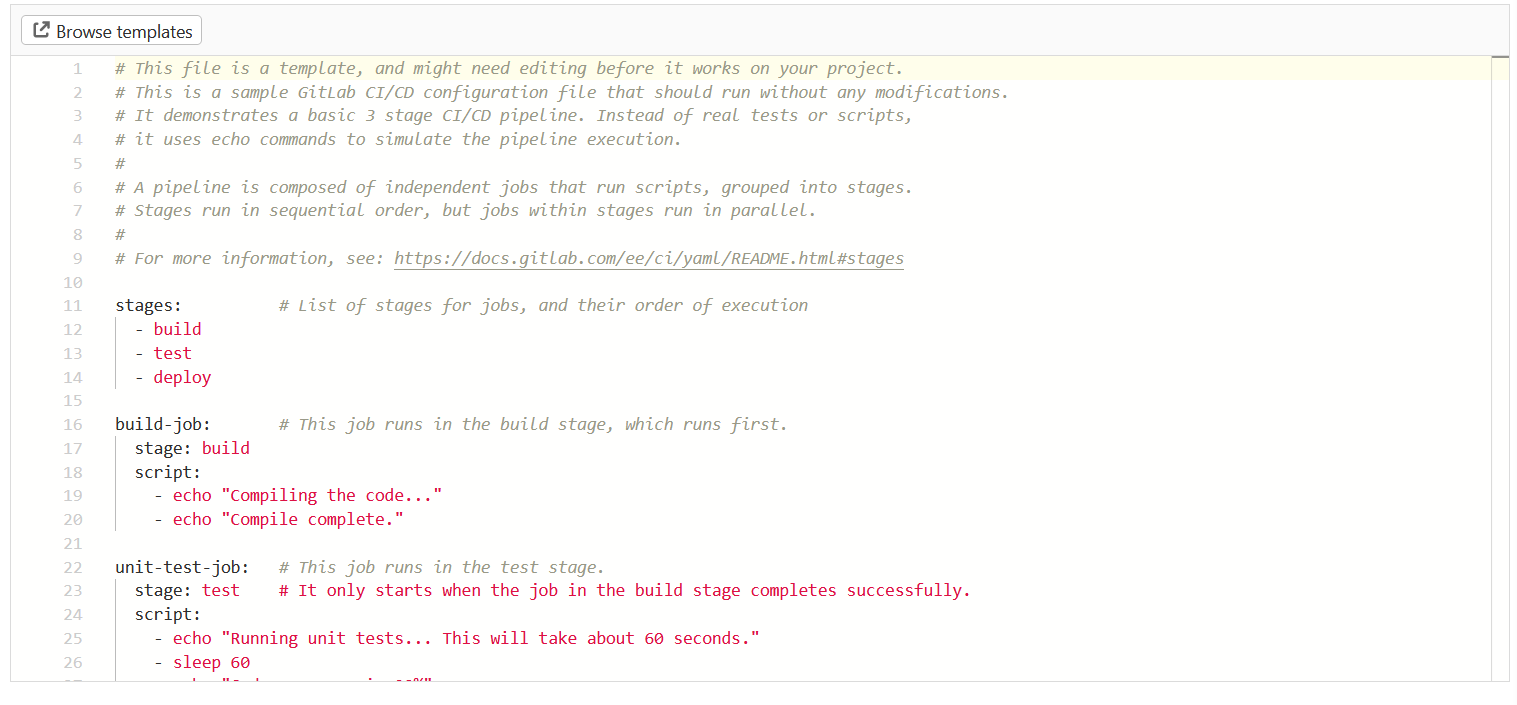

This is my .gitlab-ci.yml:

image: rocker/r-ver:4.0.3

execute:
    script:
      - apt-get update && apt-get install -y --no-install-recommends libxml2-dev
      - R -e "install.packages(c('rvest', 'magrittr', 'data.table', 'aws.s3', 'stringr', 'zoo', 'sentimentr', 'textclean', 'quanteda'))"
      - R -e "source('04_combine.R')"

This has several similarities to my Dockerfile above. The line image: docker:rocker/r-ver:4.0.3 tells Docker what image to use (similar to the FROM line in the Dockerfile).

The part under execute should look familiar from building and running our Docker image earlier. script is the name of the pipeline stage (in this case I only have one stage, so the word ‘pipeline’ is perhaps a little grand), and the following lines are terminal commands. The first two commands ensure that everything needed to run the scripts is installed, and the final one runs the processing scripts.

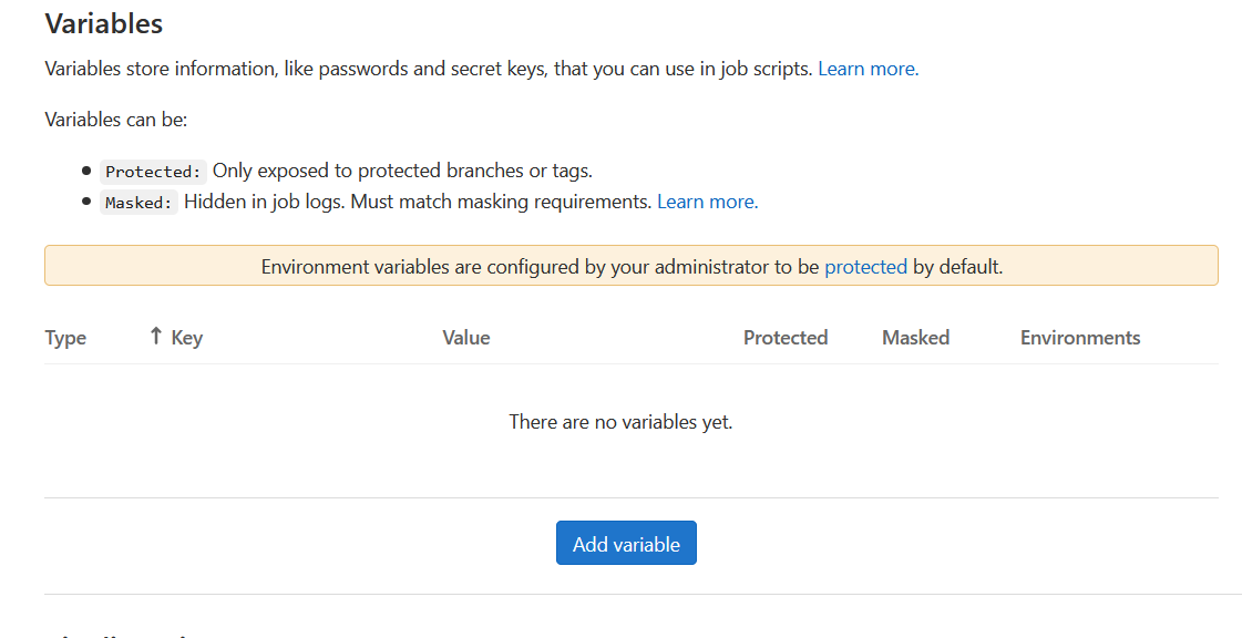
As when I was running them locally, the scripts require my AWS credentials to save generated R objects to S3. Instead of adding my credentials to GitLab and reading them from there (which would be a bad idea, particularly since this is a public repo), I added them as GitLab variables.

To do this, click ‘Settings’ in the sidebar and then ‘CI/CD’ in the expanded submenu. Under ‘Variables’, you can click ‘Add variable’ to add a key value pair. Be sure to click the checkbox ‘Protect variable’ if this is something that needs to be secret, like a password.

The final step is to schedule the pipeline to run (though ‘CI/CD’ and then ‘Schedules’ in the sidebar). Then simply add a short description and choose when you want the pipeline to run:

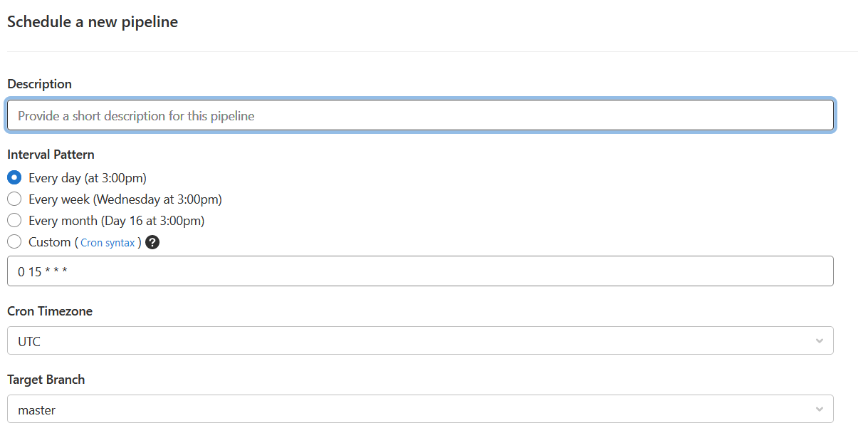
You can see the details of each time your pipeline has run though ‘CI/CD’ and then ‘Pipelines’ in the sidebar.

And with that, I no longer had to manually run my data-processing scripts (at least not for this project). A small but satisfying victory in the quest to make data pipelines take care of themselves.

Resources

I used the aws.s3 package to interact with S3 from R.
This guide by Ben Gorman on using S3 with R has a very clear walkthrough of how to set up S3 and how to use the aws.s3 package to save and load data from S3.
Colin Fay’s post on using R and Docker is great for getting started with Docker.